Welcome !!!

We hope you find our work enjoyable and interesting , where our current interest lies on using Machine Learning techniques to model sports event data. Check out our project .

Contributors: Dinesh Adhithya and Sachin Mishra

If you wish to reach out to us : Dinesh Adhithya and Sachin Mishra

1. Modelling pass difficulty/hardness in football matches.

Data Extraction and parsing

We use Statsbomb event data available at the Statsbomb github repository and collect the passes from each match to make our dataset. We have 861714 datapoints in our dataset, we need to make sure our training dataset has equal no. of completed and incomplete passes. So we select 173101 completed and Incomplete passes to form our training dataset.

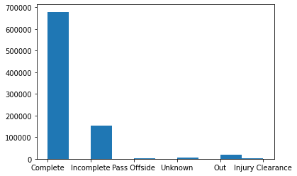
Data Exploration

pass outcome distribution of our dataset:

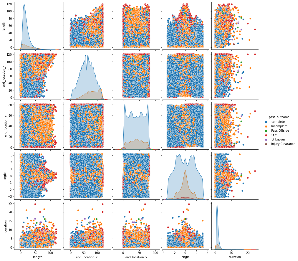
pass dataset:

Model selection

We look to model each pass using a set of features that describe a pass , namely :

1. pass length
2. pass angle
3. pass start coordinates
4. pass end coordinates
5. pass duration

We use machine learning models such as LinearRegression , Graphical Boosting models , Deep Neural Network models , etc. to predict the difficulty of a pass being completed. Each pass in training dataset is assigned 1 for a completed pass and 0 for an incomplete pass. Then such model is used on match event data to find the difficulty of passes completed during a match. A new metric called expected pass is being made by us , inspired from Xg models developed before. This metric quantifies the pass difficult which assigns each pass a value between 0 and 1 , 1 indicates a tough pass and 0 indicates an easy pass.

Deep Learning model performs at an accuracy of ~80% and is the best performing model. This model is used for application on match data.

Model Application

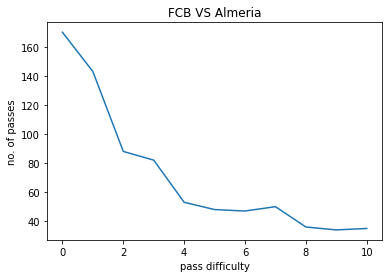
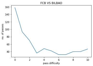
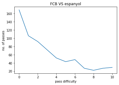
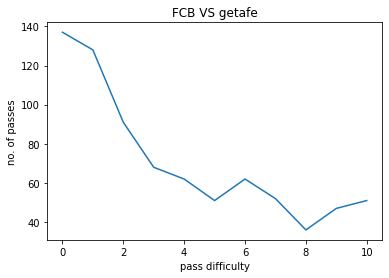
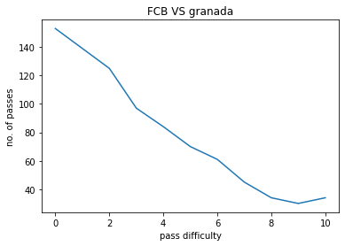
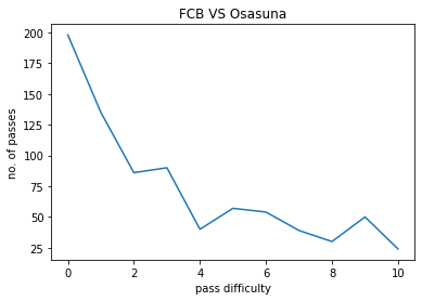
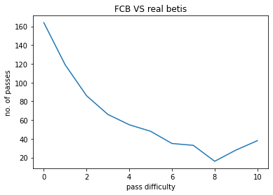
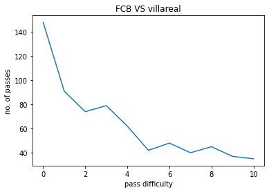
The model was used on a few matches contested by FC Barcelona , The following pass hardness distributions were obtained :

• X-axis : 0 to 10, pass hardness increases from 0 to 10.
• Y-axis : No. of passes of that particular difficulty.

FCB VS ALMERIA:

FCB VS BILBAO:

FCB VS ESPANYOL:

FCB VS GETAFE:

FCB VS GRANADA:

FCB VS OSASUNA:

FCB VS REAL BETIS:

FCB VS VILLAREAL:

A plot of pass Hardness of passes involved during a possession from the match between FCB VS Granada:

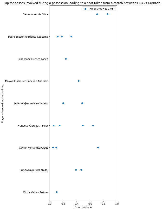
Observations

The pass difficulty histogram falls exponentially with increasing pass hardness. Passes being the most common event during football matches these plots give us an idea how risk is optimised during football matches. Passes also goes on to be the most commom type of interaction among players. Our work ponders more deeply on how a closed group of humans interact with each other and the possible application of such ideas is also being explored upon.

2. Modelling Expected Goals of shots taken during football matches using Machine Learning.

Data Extraction and parsing

We make use of Statsbomb’s open data and use ~ 13 k shots to model the probablity of a shot taken ending up as a goal.

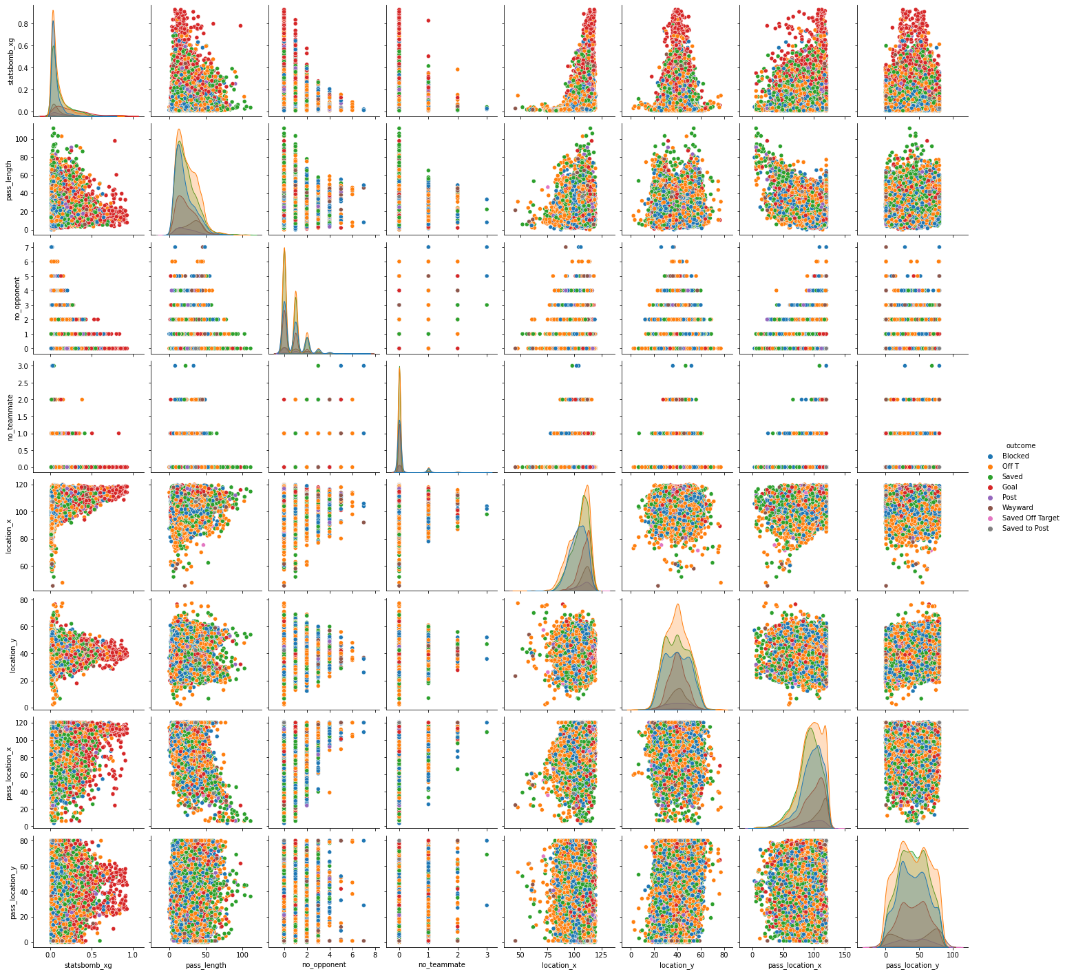
Data Exploration

shots dataset:

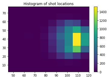
shot locations:

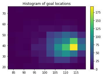
goal locations:

Model selection

The following features describing the shot were used :

1. body part from which shot was taken from.
2. technique used in the shot.
3. no. of opponents in the triangle joning the 2 end points of goal post and shot position.
4. no. of teammates in the triangle joning the 2 end points of goal post and shot position.
5. location of the shot
6. angle the shot location makes with the 2 goal posts.
7. distance from goal

The best performing ML model was deep neural networks which performed at an accuracy of ~ 87 % on testing dataset.

shot distribution plot obtained from our model:

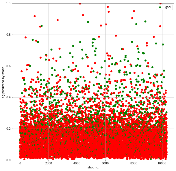
Model Application

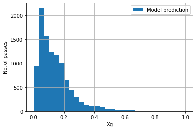
The model was applied on the testing dataset and following Xg histogram for no. of shots vs Xg was obtained and compared to Statsbomb’s Xg model.

Model prediction:

Statsbomb’s prediction:

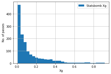
Observations

The histogram obtained by our model was in the shape of a bell curve , with maximum of the curve at an Xg of ~0.1 , whereas the statsbomb model’s curve is an exponentially falling curve whose maximum is at an Xg of 0.0. Intution suggests the curve obtained by our model makes more sense but unless a larger dataset is used for the same work we cant draw conclusions.

3. Dribble Modelling

Data Extraction and parsing

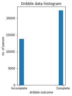
We collected ~36k dribble event data from the Statsbomb open data.

Data Exploration

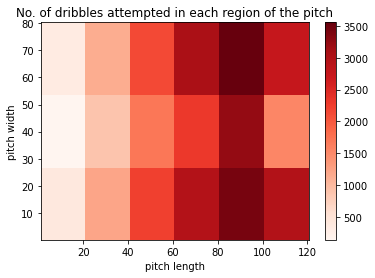
Dribble histogram:

Dribble attempted locations:

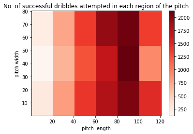
Dribble successful locations:

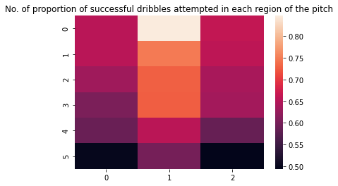
Proportion of successful dribbles:

Model selection and Application

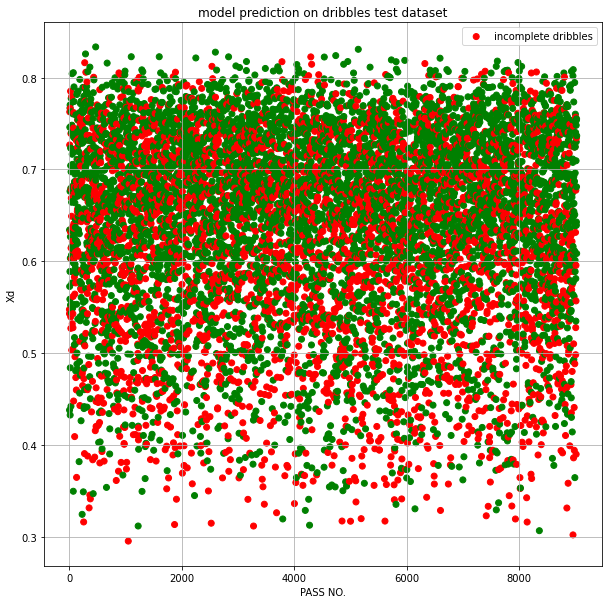
The model predicts the probability of a successful dribble , called Xd and outputs to be predicted are set as 1 for complete dribble and 0 for incomplete dribble. The best performing model had an accuracy of ~60% on the testing datasets.

Our model’s performance on testing dataset:

Observations

Dribbles have a minimum Xd of 0.113 and maximum Xd of 0.83.

Weightage to each event.

1. Avg. success rate of a dribble : 0.618
2. Avg. success rate of a pass : 0.797
3. Avg. success rate of a shot : 0.119

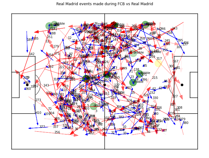
4. Model application on real match data between Real Madrid CF vs FC Barcelona on 2016-12-03

Events

The darker the color gets the harder that particular event (pass,dribbles,shots)

1. Passes -> Red
2. Carry -> Blue
3. Dribble -> Green
4. Shots from possessions -> Yellow

Madrid’s events during possession

Barcelona’s events during possession

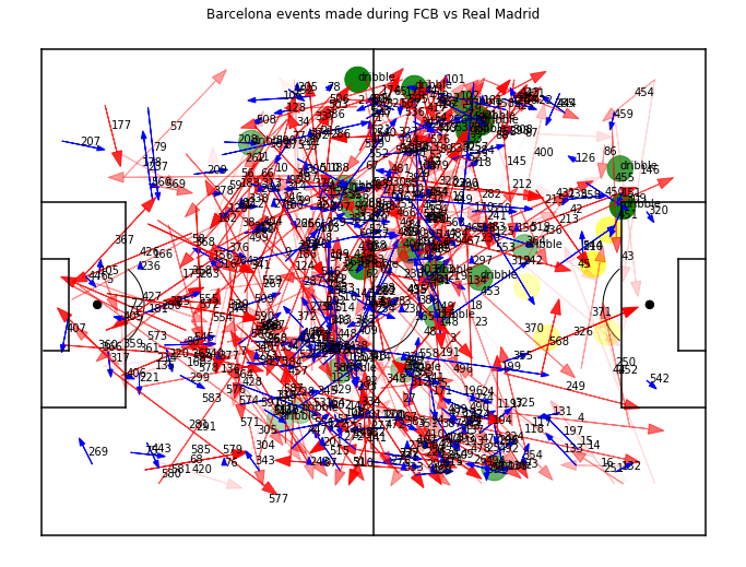
Conclusion

Inspite of performing harder passes and dribbles FCB ended with a draw , but clearly from our plots we could see which team had the better performance.

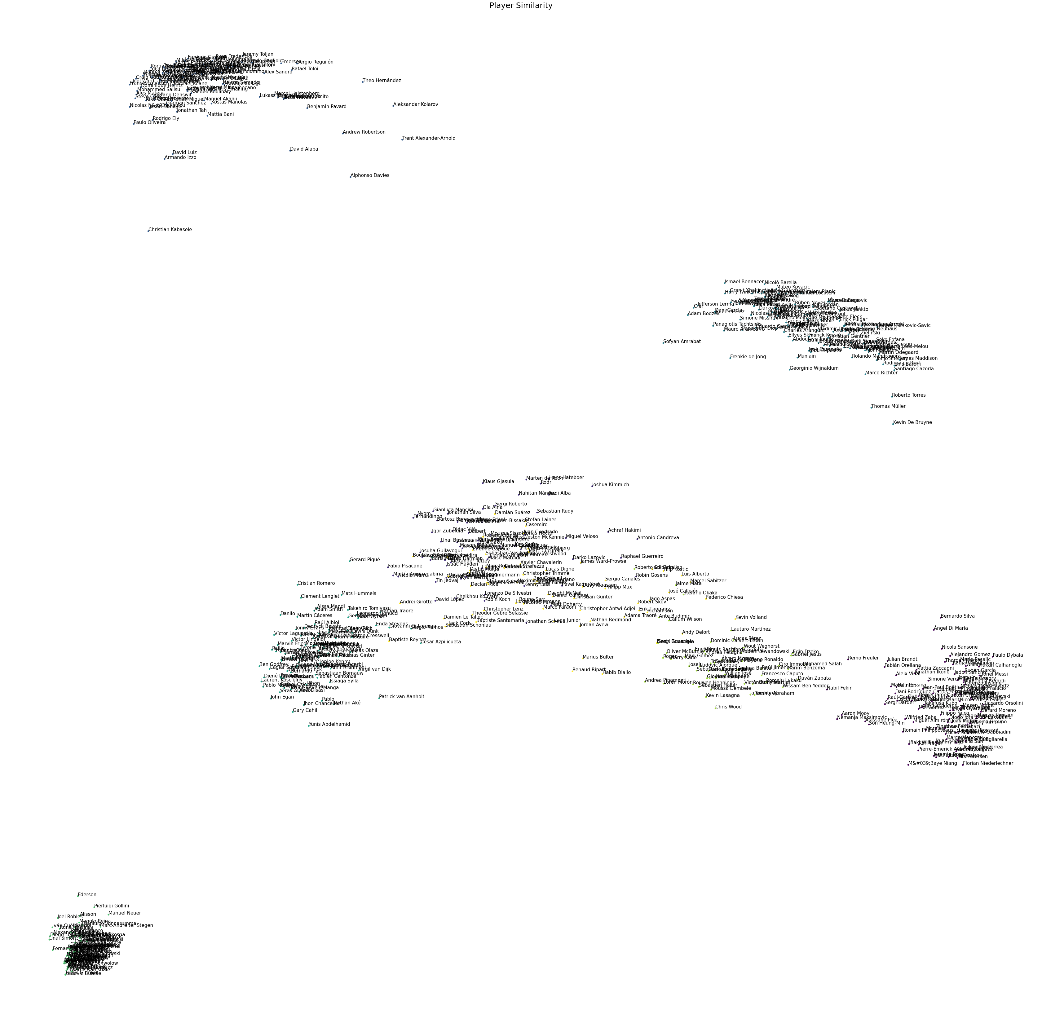
5. Clustering of football players

The data is taken from understat , and has player data of the top 5 leagues from 19/20 season. Methods such as Principal Component Analysis and k-means clustering were employed .

The followimg features describing players was used :

1. goals
2. xG
3. assists
4. xA
5. shots
6. key_passes
7. yellow_cards
8. red_cards
9. position
10. npg
11. npxG
12. xGChain
13. xGBuildup

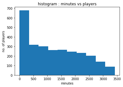
Only players who registered more than 2000 minutes were selected for the clustering process.